My journey into the world of algorithms didn’t start with a brilliant solution. It started with a spectacular failure.
As a self-taught developer, I’d reached a point where I felt I needed to get serious about the fundamentals. I was building things, sure, but I knew there was a deeper layer of understanding I was missing—the kind that separates a good developer from a great one. That layer, I decided, was algorithms.
My strategy was simple, if a bit naive: jump straight into the deep end. I created my LeetCode profile, found an easy-difficulty problem, and started coding. My first few submissions were flat-out wrong. I tweaked, I debugged, I submitted again.
Finally, after what felt like an eternity, I saw the green “Accepted” text. I felt a rush of victory, which was immediately crushed when I saw the stats: Runtime: 4481 ms. Acceptance Rate: 33%. My solution worked, but it was a disaster. It was slow, inefficient, and barely better than a third of other submissions.
That was my “aha!” moment. I realized I was trying to build a house from the roof down. I was trying to write clever code without understanding the principles that make code efficient. I was memorizing solutions without understanding the why behind them.
So, I took a step back. I put LeetCode on hold and started from scratch. I created a roadmap for learning algorithms, focusing on the fundamental foundations. This article is that roadmap for learning algorithms, the one I wish I had from day one. It’s built on three pillars that will take you from confused to confident, not by memorizing answers, but by truly understanding the concepts.
Master Complexity Analysis (The Language of Efficiency)
The Foundational ‘Why’ – Don’t Build on Sand
Before you write a single line of a sorting algorithm, before you even think about trees or graphs, you must learn Complexity Analysis. Why? Because it’s the language we use to talk about performance. Trying to solve algorithm problems without it is like trying to have a conversation without knowing the alphabet.
Complexity analysis gives us a universal way to measure an algorithm’s efficiency, completely independent of the programming language you use or how fast your computer is. It’s a predictive and strategic tool. When you understand it, you gain the ability to look at two different approaches to a problem and know which one will perform better
before you invest hours implementing the wrong one.
This isn’t just an academic exercise. Imagine you have a feature that needs to process a list of one million items. An algorithm with a complexity of O(N2) might take minutes to run, while an O(N) algorithm could finish in under a second. Learning to spot that difference upfront saves you from costly rewrites and frustrating performance bottlenecks down the line. It’s the single most important first step because it gives you the framework for making good decisions.
A Simple Analogy for Time & Space Complexity
So what are we actually measuring? We primarily look at two things: Time Complexity and Space Complexity. Let’s use an analogy: planning and cooking a big meal for friends.
- Time Complexity is the total time it takes you to cook the meal. If you’re making instant ramen for one person, it might take 3 minutes. If you have ten guests, it’ll take much longer because you have to repeat the process for each guest. The total cooking time scales with the number of guests (your input, or ‘N’). This is the measure of how an algorithm’s runtime grows as the input size increases.
- Space Complexity is the amount of memory (or pantry space) an algorithm needs to run. To cook that ramen, you need space in your shopping cart for the noodle packets and space on your counter to prepare them. As you serve more guests, you need more space for more ingredients. This is the measure of how much memory an algorithm needs as the input size grows.5
Often, these two exist in a trade-off. You might find a super-fast algorithm (low time complexity) that requires a ton of memory (high space complexity), or a very memory-efficient algorithm that takes longer to run. Understanding this balance is at the heart of engineering.
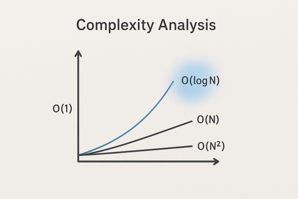
A Practical Guide to Big O Notation (The Ruler of Efficiency)
The language we use for complexity is called Big O notation. Big O describes the growth rate of an algorithm’s complexity as the input size (N) gets very large. Crucially, it focuses on the worst-case scenario. This gives us a reliable upper bound on performance, so we know our algorithm will never perform worse than this.
To keep things simple, Big O follows two main rules:
- Drop the Constants: An algorithm that runs 2N steps is simplified to O(N). As N gets huge, the ‘2’ becomes insignificant.
- Drop Non-Dominant Terms: An algorithm that takes N2+N steps is simplified to O(N2). The N2 term grows so much faster than N that it’s the only one we care about for large inputs.
Let’s break down the most common Big O notations you’ll encounter.
O(1) — Constant Time
- Analogy: Finding a book in a library using its exact ISBN number. No matter if the library has 100 books or 10 million, the task takes the same amount of time.
- Explanation: The performance is always the same, regardless of the input size. It’s the holy grail of efficiency.
- Code Example: Accessing the first element of an array.
# This function's runtime doesn't depend on the size of the list.
def get_first_element(numbers):
    return numbers
O(logN) — Logarithmic Time
- Analogy: Looking up a word in a physical dictionary. You don’t start at ‘A’ and read every word. You open it to the middle, see if your word comes before or after, and then discard half the book. You repeat this, halving the search space each time.
- Explanation: The runtime grows very slowly as the input size increases. This is because you eliminate a large portion of the data with each step.
- Code Example: Binary Search.
# With each step, we cut the search space in half.
def binary_search(sorted_arr, target):
    low, high = 0, len(sorted_arr) - 1
    while low <= high:
        mid = (low + high) // 2
        if sorted_arr[mid] == target:
            return mid
        elif sorted_arr[mid] < target:
            low = mid + 1
        else:
            high = mid - 1
    return -1
O(N) — Linear Time
- Analogy: Reading every single page of a book from start to finish. If the book doubles in length, the time it takes you to read it also doubles.
- Explanation: The runtime grows in direct proportion to the size of the input. This is a very common and generally acceptable complexity.
- Code Example: Searching for an item in an unsorted array.
# In the worst case, we have to check every single element.
def linear_search(arr, target):
    for item in arr:
        if item == target:
            return True
    return False
O(NlogN) — Linearithmic Time
- Analogy: This one is a bit more abstract, but think of it as the efficiency of a professional sorting service for a massive pile of documents. They use a smart “divide and conquer” strategy (the log N part) on all the documents (the N part).
- Explanation: This is a hallmark of highly efficient sorting algorithms. It performs significantly better than O(N2) for large datasets.
- Code Example: Merge Sort.
# This isn't the full code, but it shows the recursive structure.
def merge_sort(arr):
    if len(arr) <= 1:
        return arr
    mid = len(arr) // 2
    left_half = merge_sort(arr[:mid])
    right_half = merge_sort(arr[mid:])
    # The magic happens in merging the sorted halves.
    return merge(left_half, right_half)
O(N2) — Quadratic Time
- Analogy: Shaking hands with every single person in a large room. For each of the N people, you have to shake hands with the other N−1 people. The number of handshakes grows very quickly as more people enter the room.
- Explanation: The runtime grows exponentially with the input size. This is often caused by nested loops and can become very slow, very fast.
- Code Example: A simple (and inefficient) sorting algorithm like Bubble Sort.
# The nested loop gives this algorithm its O(N^2) complexity.
def bubble_sort(arr):
    n = len(arr)
    for i in range(n):
        for j in range(0, n - i - 1):
            if arr[j] > arr[j + 1]:
                arr[j], arr[j + 1] = arr[j + 1], arr[j]
To help you keep these straight, here is a quick cheat sheet.
| Notation | Common Name | Performance | Real-World Analogy |
| O(1) | Constant | Excellent | Finding a book by its ISBN number. |
| O(logN) | Logarithmic | Great | Looking up a word in a dictionary. |
| O(N) | Linear | Good | Reading every page of a book. |
| O(NlogN) | Linearithmic | Good | The efficiency of a professional sorting service. |
| O(N2) | Quadratic | Poor | Shaking hands with everyone in a large crowd. |
The goal here is not to memorize formulas, but to develop an intuition. When you see a nested loop, your brain should whisper “O(N2)”. When you see a problem on a sorted array, you should think “O(logN) might be possible.” This intuition is the true foundation.
Build Your Toolbox of Core Data Structures
The Craftsman’s Analogy – Choosing the Right Tool
Once you can speak the language of efficiency, the next step is to get to know your tools. A data structure is simply a way of organizing and storing data so that it can be accessed and manipulated efficiently. Think of a great developer as a master craftsman. They have a toolbox filled with specialized tools, and they know exactly which one to use for which job.
Your choice of data structure is a direct consequence of understanding complexity. An Array gives you lightning-fast access to an element if you know its index (O(1)), but inserting an element in the middle is slow (O(N)) because you have to shift everything over. A Linked List, on the other hand, is slow for access (O(N)), but incredibly fast for insertions and deletions in the middle (O(1)) if you already have a pointer to that location.
Using an Array when you need frequent insertions is like trying to hammer a nail with a screwdriver. It might work eventually, but it’s messy, inefficient, and shows you don’t understand your tools. Knowing the built-in strengths and weaknesses of each data structure is what enables elegant and efficient problem-solving.
The Essential Toolkit: A Quick Reference Guide
Here are the essential “tools” every developer should have in their toolbox.
- Array & String: An Array is a collection of items stored in a neat row in memory, making it perfect for when you need fast, indexed access to elements and the collection size is relatively stable. A String is essentially a specialized array of characters.
- Stack: A “Last-In, First-Out” (LIFO) structure, like a stack of plates where you take the top one first, which is best for managing tasks that need to be reversed, like the “undo” function in a text editor.
- Queue: A “First-In, First-Out” (FIFO) structure, like a line at a ticket counter, which is ideal for processing tasks in the order they were received, such as managing a printer queue.
- HashMap / HashSet:
-
- HashMap: A structure that stores key-value pairs, like a real-world dictionary, providing nearly instant (O(1) on average) lookups, making it perfect for quickly finding data associated with a unique identifier.
- HashSet: A structure that only stores unique items, like a gym’s check-in system that just verifies if a member ID is valid, which is best for when you just need to quickly check for the existence of an item in a collection with no duplicates.
- Linked List: A sequence of nodes where each node points to the next, like a train where the cars are linked together, making it best for dynamic lists that require frequent insertions and deletions in the middle.
- Heap (Min/Max): A specialized tree-based structure that always keeps the smallest (Min-Heap) or largest (Max-Heap) element at the root, making it the perfect tool for implementing a priority queue, like an emergency room triage system that always treats the most critical patient first.
- Tree (Basics): A hierarchical structure with a root and child nodes, like a family tree or a computer’s file system, which is best for representing any kind of hierarchical relationship.
- Graph (Basics): A collection of nodes (vertices) connected by edges, like a map of cities and roads or a social network, which is best for modeling complex, interconnected relationships where there is no clear hierarchy.
This quick reference table can help you visualize which tool to reach for.
| Data Structure | What It Is (In One Sentence) | Best For… |
| Array / String | A fixed-size, ordered list of elements in a row. | Fast random access by index. |
| Stack | A “Last-In, First-Out” (LIFO) collection. | Reversing things, like an “undo” button. |
| Queue | A “First-In, First-Out” (FIFO) collection. | Processing items in the order they arrive. |
| HashMap | A collection of key-value pairs (like a dictionary). | Lightning-fast lookups, insertions, and deletions. |
| HashSet | A collection of unique items. | Checking for the existence of an item, no duplicates. |
| Linked List | A dynamic chain of elements linked together. | Frequent insertions and deletions in the middle. |
| Heap | A structure to always have the min/max at the top. | Implementing a priority queue (e.g., ER triage). |
| Tree | A structure for hierarchical data (parent-child). | Representing file systems or organizational charts. |
| Graph | A structure for interconnected data (nodes & edges). | Modeling networks like social media or maps. |
Learn the Problem-Solving Patterns (The “Moves”)

Patterns Over Memorization – Learning the Chess Moves
You now understand how to measure efficiency (Pillar 1) and you have your toolbox of data structures (Pillar 2). The final pillar is about technique: learning the “moves.”
A common trap for beginners is trying to memorize the solution to every problem they see. This is not just impossible; it’s counterproductive. The real goal is to recognize that most algorithmic problems are just variations of a handful of underlying patterns.
An experienced developer doesn’t see 500 unique problems; they see 10-15 patterns repeated in different contexts. Learning these patterns is like learning the fundamental moves in chess. Once you know how a “fork” or a “pin” works, you can apply it in thousands of different game situations. These patterns are the meta-skill that ties everything together.
Four Foundational Patterns Explained
Let’s look at four of the most powerful and common patterns you’ll encounter.
1. The Two Pointers Pattern
- What it is: A brilliantly simple technique for problems on sorted arrays or lists. You initialize two pointers, often at opposite ends of the array, and move them towards each other based on some condition. This allows you to efficiently process pairs of elements.
- Analogy: Imagine two friends starting at opposite ends of a bridge and walking towards each other to meet in the middle. Their combined movement efficiently covers the entire bridge without either person having to walk the full length back and forth.
- What it solves: It’s perfect for problems like “find a pair of numbers in a sorted array that adds up to a target.” A brute-force approach would be O(N2), but the Two Pointers pattern solves it in a single pass, achieving an elegant O(N) solution.
2. The Sliding Window Pattern
- What it is: A technique for efficiently processing contiguous subarrays or substrings. You create a “window” over the data, and as you “slide” it along the array, you intelligently update your calculations by adding the element that enters the window and subtracting the one that leaves.
- Analogy: You’re on a train looking at a long fence. Your field of view is the “window.” As the train moves, new fence posts come into view on one side as old ones disappear on the other. You’re taking in the whole scene without having to stop and re-scan the entire fence every second.
- What it solves: It’s ideal for problems like “find the maximum sum of any contiguous subarray of size K” or “find the longest substring with no repeating characters.” It turns a potential brute-force mess into a clean, linear-time O(N) solution.
3. The Binary Search Pattern
- What it is: A classic “divide and conquer” algorithm for finding an element in a sorted array. It works by repeatedly comparing your target value to the middle element of the current search space. Based on the comparison, you eliminate half of the remaining elements and repeat the process on the half that could contain the target.
- Analogy: The classic “guess the number” game. Someone thinks of a number from 1 to 100. Your first guess is 50. They say “higher.” You’ve just eliminated 50% of the possibilities. Your next guess is 75, and so on. You find the number incredibly quickly by halving the possibilities with each guess.
- What it solves: Any problem that requires finding an item in a sorted list or array. It’s incredibly efficient, with a time complexity of O(logN).
4. The Recursion & Backtracking Pattern
- What it is:
-
- Recursion: A process where a function calls itself to solve smaller, identical versions of the main problem, until it reaches a simple “base case” that can be solved directly.
- Backtracking: An algorithm that uses recursion to explore all possible solutions to a problem. When it hits a path that won’t lead to a solution, it “backtracks” (or undoes its last choice) and tries another path.
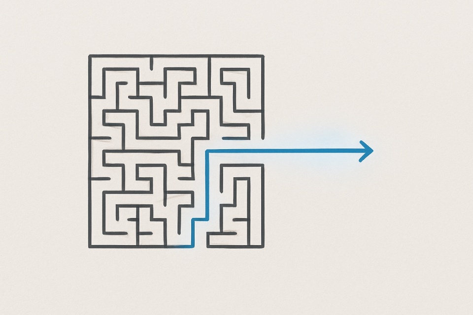
- Analogy: Solving a maze.You go down one path (this is the recursive step). If you hit a dead end, you turn around and go back to the last intersection to try a different path (this is backtracking). You continue this process of exploring and backtracking until you find the exit.
- What it solves: Complex problems involving permutations, combinations, and exploring all possible configurations, like solving a Sudoku puzzle or generating all valid sets of parentheses.
Conclusion: Build the Foundation, Then Climb the Mountain
Looking back at my first, failed LeetCode submission—that agonizing 4481 ms runtime—I realize now that it wasn’t a measure of my ability as a developer. It was a predictable outcome of trying to climb a mountain without a map, a compass, or even proper boots. I was trying to run before I could walk.
The intimidating world of “algorithms” isn’t a single, monolithic mountain. It’s a landscape that can be navigated with the right tools and a clear path. The three pillars of this roadmap for learning algorithms, mastering Complexity Analysis, building your Data Structures toolbox, and learning the Problem-Solving Patterns, are that path. They are the foundation upon which all elegant, efficient, and clever solutions are built.
Stop the cycle of jumping into the deep end and feeling like you’re drowning. Take a step back. Build your foundation, one pillar at a time. The climb will be challenging, but with the right roadmap for learning algorithms, you’ll find yourself reaching heights you never thought possible.
I’m Reza Ghaderipour, and I share my insights about Technology and Strategy.
What has your learning journey been like? Share your own “aha!” moments or struggles in the comments below. Let’s learn together!